The purpose of this exercise was to make a graph with the world map. We also learned how to implement a for loop.

We first load in our file. We will then need code from the three libraries, tidyverse, lubridate, and maps, so we call them next.

monthly_temps <- read.csv("monthly_global_land_and_ocean_temperature_anomalies.csv")

library(tidyverse)
library(lubridate)

## 
## Attaching package: 'lubridate'

## The following object is masked from 'package:base':
## 
##     date

library(mapproj)

## Loading required package: maps

## 
## Attaching package: 'maps'

## The following object is masked from 'package:purrr':
## 
##     map

We then mutate our monthly_temps data object to get in useable form. Since the day is missing from our date, we truncate it to not include that number in the date. We then modify our object to seperate the year and the month into seperate objects, instead of one date object. We set label = TRUE to include the names of the months, but only their abbreviations. We want to rename our Value column to temperature_anomaly so that the column more clearly states what it is showing. We also choose to drop the YearMonth column because we no longer need it.

monthly_temps <- mutate(monthly_temps, date = ymd(YearMonth, truncated=1))

monthly_temps <- mutate(monthly_temps,
                        year=year(date),
                        month=month(date,label=TRUE))

monthly_temps <- rename(monthly_temps, temperature_anomaly = Value)

monthly_temps <- select(monthly_temps, -YearMonth)

We save our work to a csv file. We also save an R version to make sure to preserve the classes of our data. We also read in the gridded_data.csv file to complete our final graph. From the gridded_data file, we divide the rows of the file by 37 to give us how many months we have in total because currently each month takes up 37 rows in the data file. We create an empty list to then put our months into. We then use a for loop to cycle through all of our objects.

write_csv(monthly_temps, path="modified_monthly_temps.csv")
save(monthly_temps, file="monthly_data.RData")


gridded_data <- read.csv("gridded_data.csv", header = F)

number_of_months <- nrow(gridded_data)/37

monthly_data <- vector("list", number_of_months)

for(i in 1: number_of_months){monthly_data[[i]] <- gridded_data[((i-1)*37+2):(i*37),] #extract and store temperature
          integer_date <- gridded_data[((i-1)*37+1),2]*100+gridded_data[((i-1)*37+1),1] #get date
          current_date <-ymd(integer_date,truncated=1) #convert to date            
          current_month <-month(current_date,label=T)
          current_year <-year(current_date)
          names(monthly_data)[i] <- paste(current_month, current_year)
}

We create a second for loop to enter our objects in our current_data object and then after they’ve cycled through, we refill our monthly_data object.

for(i in 1: number_of_months){current_data <- monthly_data[[i]]
          latitudes <- rev(seq(from= -87.5, to=87.5, by=5))
          current_data$latitude <- latitudes
          longitudes <- seq(from= -177.5, to=177.5, by=5)
          colnames(current_data)[1:72] <- longitudes
          current_data <- gather(current_data, key="longitude", value="TempAnom", -latitude)
          current_data$longitude <- as.numeric(current_data$longitude)
          current_data <- mutate(current_data, TempAnom = ifelse(TempAnom==-9999, NA, TempAnom/100))
          monthly_data[[i]] <- current_data 
}

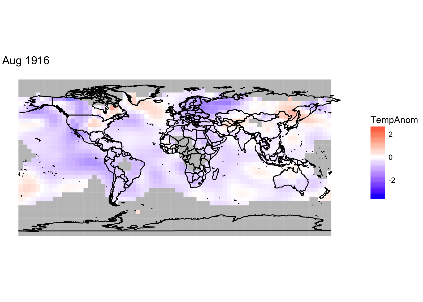
For our graph, we want to display a map of the world (which we got from the mapproj library), so we save a world object. We use August 1916 as a tester date. We assign current_data to this tester date.

world <- map_data("world")


current_month <- "Aug 1916"


current_data <- monthly_data[[current_month]]


current_name <- names(monthly_data[current_month])

We assign our graph to an object so that we can further manipulate it. We also add the geom_path function to our graph to display the world map. The albers function determines the scale of the world we are looking at and we then show that choosing 123 gives us the same result as choosing Aug 1916 because this is the 123rd month in the data set. Finally, we save all of our work into the data file climate_data.RData to store it.

g<-ggplot()+ geom_tile(data=current_data, aes(x=longitude, y=latitude, fill=TempAnom),
                       width=5, height=5,alpha=.5)+
  scale_fill_gradient2(low="blue",mid="white",high="red",midpoint=0)+
  theme_void()+labs(title=current_name)

g <- g+geom_path(data = world, aes(x = long, y = lat, group = group))

g + coord_map("albers",parameters=c(0,0))

current_month <- 123

save(monthly_data, monthly_temps,file="climate_data.RData")